This is the draft website for Programming Historian lessons under review. Do not link to these pages.
For the published site, go to https://programminghistorian.org
Contents
- Calibrating Radiocarbon Dates with R
- The Basic Principles of Radiocarbon Dating
- Why Calibrate Radiocarbon Dates?
- How to Calibrate?
- Applications with R
- Conclusion
- Endnotes
- Bibliography
Calibrating Radiocarbon Dates with R
Since its discovery and the revolution that followed, the radiocarbon dating method has become common practice for archaeologists and historians. This is because it either constitutes the only source of chronological information, or because it complements other sources, whether they be material or textual.
The purpose of this lesson is to learn how to calibrate individual radiocarbon dates, combine several dates into one, and then test for differences. The radiocarbon method is a so-called “absolute”1 dating method, which has its own time frame. So, calibration is an essential step to this process, since it allows us to translate from a radiocarbon date of reference to a calendar date of reference.
This lesson will show you how to calibrate radiocarbon dates with R. Using R allows you to set up data processing routines and guarantees the reproducibility of your results at the time of their publication. This lesson assumes that you are comfortable with the basic use of R and understand basic concepts of statistics.2 This lesson is limited to simple calibration cases and does not cover advanced cases (for example, marine calibration, reservoir effects, etc.) nor Bayesian chronological modeling problems.
The Basic Principles of Radiocarbon Dating
Proposed in the late 1940s by Willard Libby and his colleagues,3 the radiocarbon method uses the radioactive decay of carbon-14 (14C) to construct a chronometer. This makes it possible to estimate dates, i.e. time intervals measured from the present.4 By convention, radiocarbon dates are thus expressed in (kilo) years BP (Before Present, before 1950).5
To develop a chronometer, three necessary conditions must be met:
- The chosen phenomenon must follow a law which varies over time;
- The law in question must be independent of environmental conditions;
- An initial event must be able to be determined.
14C is one of three isotopes of carbon, along with 12C and 13C. 14C is a radioactive isotope: it tends to disintegrate over time according to a decreasing exponential law. It is a nuclear phenomenon, independent of the environment. For any given isotope, this phenomenon of radioactive decay can be described using a particular quantity, the “radioactive half-life” (denoted \(T\), also called “half-life”). The latter corresponds to the time necessary for the disintegration of half of the initial quantity of atoms.
The half-life of14C is 5,730 ± 40 years: for an initial quantity \(N_0\) of 14C atoms, \(\frac{N_0}{2}\) remains after 5,730 years, \(\frac{N_0}{4}\) after 11,460 years, etc. (fig. 1). After 8 to 10 half-lives (around 45,000 to 55,000 years), the quantity of 14C to be too low to be measured: this is the limit of the method.
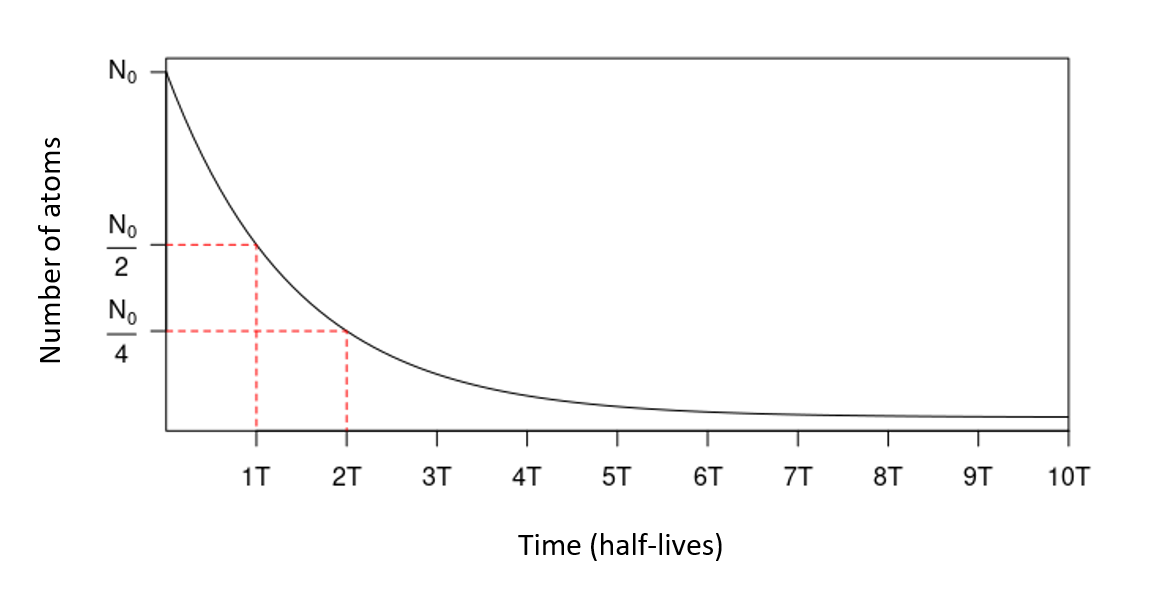
Figure 1. Exponential decay of an initial quantity of radioactive atoms, over time (expressed in number of half-lives.)
Carbon-14 is produced naturally in the upper atmosphere through the effect of cosmic radiation. It is then gradually absorbed by living organisms throughout the trophic chain, starting with photosynthetic organisms. The 14C content in living organisms is constant and in equilibrium with the atmospheric content.6
When an organism dies, exchanges with its environment stop. Assuming that there is no external contamination, we consider this a close system: radioactive decay is the only phenomenon affecting the quantity of 14C contained in the organism’s body. Therefore, the event dated by the radiocarbon is the death of the organism.
Unless we specifically are looking for when an organism died, the radiocarbon date can give a terminus ante or post quem for the archaeological event that we wish to position in time. In other words, this is the moment before or after which the archaeological or historical event of interest took place (for example, the abandonment of an object, combustion of a hearth, deposition of a sedimentary layer, etc.) depending on available contextual elements, like stratigraphy. These contextual elements are important as they help us interpret the results; in particular, they help us ensure the absence of taphonomic problems, and that there is indeed a direct relationship between the dated sample and the event of interest.7
Thanks to the law of radioactive decay, if we know the initial quantity \(N_0\) of 14C contained in an organism at its death (time \(t_0\) and the remaining quantity of 14C at time \(t\)), it is possible to measure the time elapsed between \(t_0\) and \(t\): the radiocarbon date of an archaeological object.
- The current amount of 14C in an object can be determined in the laboratory, either by counting the 14C nuclei or by counting the number of decays per unit of time and per amount of matter (specific activity).
- To determine the initial quantity, the radiocarbon method is based on the following hypothesis: the quantity of 14C in the atmosphere is constant over time and equal to the current content.
This initial premise allowed Libby and his colleagues to demonstrate the feasibility of the method, by carrying out the first radiocarbon dating on objects of known age.8 From these results, it appears that there is a linear relationship between the radiocarbon dates measured and the calendar dates obtained by other methods (fig. 2A).
Why Calibrate Radiocarbon Dates?
However, a challenge arose: studies carried out in the second half of the 20th century, as older and older objects were dated, showed an increasingly significant gap between the measured age and the expected age.
Contrary to Libby’s premise, the 14C content in the atmosphere is not constant over time, which partly explains the observerved differences. The atmospheric 14C content varies depending on natural phenomena (variations in the earth’s magnetic field, solar activity, volcanic activity, carbon cycle, etc.) and anthropogenic phenomena. These phenomena can be contradictory: the use of fossil fuels releases very old carbon, and tends to reduce the relative content of 14C (Suess effect); conversely atmospheric nuclear tests have produced large quantities of 14C.
The chronometer given to us by the radiocarbon method therefore does not have a regular pattern, because the atmospheric 14C content varies over time. Consequently, radiocarbon dates (we will subsequently use the expression “conventional dates”, see figures 2A and 2B on the y-axis) belong to a reference frame that is specific to them.
The use of Libby’s premise nevertheless remains the only accessible way to estimate the initial quantity of 14C at the closure of the system. It is therefore necessary to carry out a calibration operation to transform a conventional date into a calendar date. This operation is carried out using a curve,9 the values for which are regularly updated by the scientific community.10 The calibration curve is constructed by thus providing an equivalence table between radiocarbon time and calendar time (fig. 2B).
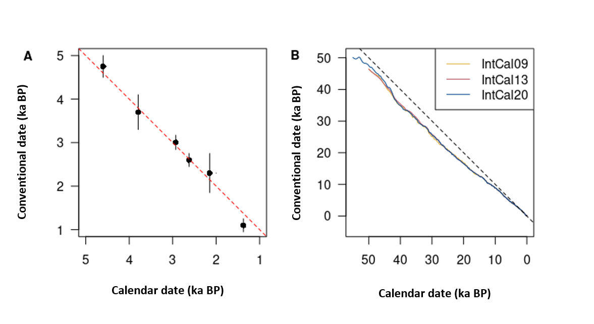
Figure 2. Dates measured by radiocarbon based on expected calendar dates. (A) Curve of Knowns, radiocarbon dates of archaeological objects whose calendar date is known by independent methods (after Arnold and Libby, 1949). The 1:1 line, for which a conventional date is equal to a calendar age, is shown as a dashed line. (B) IntCal09, IntCal13 and IntCal20 calibration curves (Reimer et al. 2009, 2013 and 2020). The difference to the right 1:1 (dashes) is all the more marked as the dates are older.
How to Calibrate?
We have just seen that it was necessary to calibrate radiocarbon dates. On paper, the calibration process is fairly simple, thanks to the conversion table between radiocarbon time and calendar time. In this way, the calibration process is complicated by taking into account the errors inevitably associated with physical measurements.
A conventional date (noted here as \(t\)) is the result of a measurement and, as there is no perfect measurement, it is always accompanied by a term corresponding to the analytical uncertainty (\(\Delta t\)) and expressed in the form \(t \pm \Delta t\) (date, plus or minus its uncertainty). This uncertainty results from the combination of different sources of error within the laboratory: it is a random uncertainty inherent to the measurement.
A conventional date is thus an estimator of the true radiocarbon date of the dated object. If the dating of the same sample is repeated a very large number of times, its value is likely to vary and there is very little chance that it will coincide exactly with the true radiocarbon date. So it is preferable to focus on an interval which is highly probable to contain the real (unknown) value of the conventional date. In this way, uncertainty characterizes the dispersion of values that could reasonably be attributed to the true date. A conventional date is the realization of a random process, radioactive decay, and can be modeled using a particular probability law: normal distribution.11
Only two parameters are necessary to characterize the distribution of values according to a normal law: the mean \(\mu\) (central tendency) and the standard deviation \(\sigma\) (dispersion of values). The properties of the normal distribution are such that the interval defined by \(\mu \pm \sigma\) contains 67% of the values. If we multiply the standard deviation by two, the interval \(\mu \pm 2\sigma\) contains 95% of the values (fig. 3).
So, if we express the uncertainty of a conventional date as a function of the standard deviation, there is a 68% chance that the interval at \(1\sigma\) contains the real conventional date. Likewise, the interval at \(2\sigma\) has a 95% chance of containing the true conventional date. The interval at \(1\sigma\) is less dispersed, but it has less chance of being correct than at \(2\sigma\). The range of values retained is narrower, but it is less likely to contain the real conventional date.
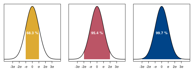
Figure 3. Normal distribution with mean 0 and standard deviation 1 with normality ranges at 68%, 95% and 99% confidence levels. The distribution of values is such that the dispersion is symmetrical around the central tendency.
The simplest approach for calibrating a radiocarbon date consists of intercepting the calibration curve between the uncertainty bounds (\(t - \Delta t\) and \(t + \Delta t\) in the \(1\sigma\) case) to obtain the correspondng calendar age interval. This is shown in Figure 4, which shows the calibration of a conventional date by intercepting a calibration curve whose uncertainty is represented by a gray band. Conventional and calendar dates are shown at \(1\sigma\) (black bands) and \(2\sigma\) (hatched bands).
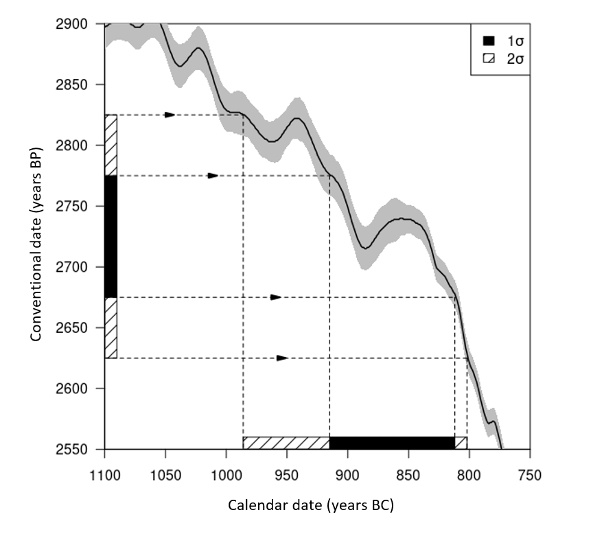
Figure 4. Calibration of a conventional age of 2725 ± 50 years BP by interception of the IntCal20 calibration curve.
However, this approach does not take into account the fact that a radiocarbon date is described by a normal distribution. In the range defined by the radiocarbon date, plus or minus its uncertainty, not all values have the same probability of coinciding with the true radiocarbon date, but calibration by simple interception assumes the opposite. Therefore, the approach widely used now12 also consists of taking into account the normal distribution of radiocarbon dates. We sometimes use the expression “probabilistic calibration” to refer to this. This calibration method uses numerical methods and the resulting distribution of calendar dates is not equally likely (fig. 5).
It is easy to describe a conventional date and its uncertainty with a normal law; but this cannot be done with a calendar date once calibrated. Due to the oscillations of the calibration curve, it is actually not possible to describe the distribution of a calendar date with a specific probability law, as can be seen in Figure 5. Thus, a calibrated date has to be described as an interval.
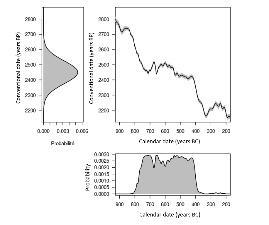
Figure 5. Distributions of a radiocarbon age of 2450 ± 75 years BP before and after calibration, respectively top left and bottom right. Top right: extract from the IntCal20 calibration curve (solid line) and associated error (gray band).
The interval to which a calendar date belongs results from the uncertainty of the conventional date, from the shape of the calibration curve, and from the uncertainty associated with the latter. This interval, between the limits of which the calendar date has a given probability of being included, can be obtained in two distinct ways (fig. 6):
- Highest Posterior Density Interval (HPDI): the limits of the interval correspond to the regions of the distribution whose cumulative probability is greater than a given threshold.
- credibility interval: the limits of the interval correspond to the quantiles of the distribution.
When the distribution of a calibrated date is multimodal, the interval at highest densities often corresponds to the union of several disjoint intervals, unlike the credibility interval which always provides a continuous range of values.13 The higher density interval is therefore often more informative, which is why it is commonly used to present calibrated results.
There are periods which are more or less suitable for radiocarbon dating, depending on the shape of the curve. The least favorable case is the existence of plateaus in the calibration curve. A typical case is the Iron Age plateau (fig. 5). For example, a conventional date of 2,450 ± 75 years BP corresponds, once calibrated to 95% (HPD interval), to a calendar age between 2,719 and 2,353 years BP (i.e. 769-403 BCE). Thus, despite a conventional age with a fairly low uncertainty (3%), the corresponding calendar age has a 95% chance of being found in a time interval which covers almost the entire early Iron Age (fig. 5). By performing the calibration at 68% (HPD interval), we are confronted with another problem linked to oscillations of the calibration curve. A calendar date has a 68% chance of belonging to the union of the intervals 748-684 (18%), 665-637 (8%), 586-580 (2%), 568-452 (32%) and 444-415 (8%) BCE and not at a single interval (fig. 6).
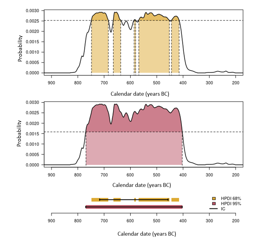
Figure 6. Estimation of calibrated intervals. The top two graphs illustrate the estimate of the highest density regions at 68% and 95%. The bottom graph allows you to compare the HPD intervals thus obtained and the corresponding credibility intervals (solid lines).
In some situations, it is common to keep calibrated dates expressed in years BP. In this case it is recommended to specify cal BP to avoid any confusion for the reader. These calendar ages in years BP can be converted to dates expressed before or after our era (BC/AD, before Christ/anno Domini). To do this, simply use the following calculation rule:
To convert a calibrated age (noted \(x\)) expressed in years BP into years BC/AD, knowing that there is no year 0 in the Gregorian calendar:
- If the calibrated age is less than 1950 BP: \(1950 - x\) AD
- If the calibrated age is greater than or equal to 1950 BP: \(1949 - x\) BC
By now it is clear that these details, if poorly understood, can quickly lead to overinterpretations. So when publishing a dating series, it is important to present all the data and choices that contributed to obtaining our calendar dates. The use of free tools promotes both transparency and reproducibility of results, which are two very important aspects with regard to the calibration of radiocarbon dates.
Applications with R
Many tools are now available to calibrate radiocarbon dates, like OxCal, CALIB and ChronoModel. But these tools are rather intended to deal with Bayesian modeling problems of chronological sequences (which we don’t cover in this lesson). R offers an interesting alternative to these tools which suits our needs. R is distributed under a free license, promotes reproducibility and lets us integrate the processing of radiocarbon date into larger projects (spatial analysis, etc.).
Several R packages help us carry out radiocarbon date calibration. (Bchron, oxcAAR, etc.) are often oriented towards modeling (constructing chronologies, age-depth models, etc.). The package we will use in this lesson is called rcarbon (Bevan and Crema 2020). It allows us to easily calibrate and analyze radiocarbon ages.
Case Study
In order to concretely address the question of calibrating radiocarbon ages, let us look at the example of dating the Shroud of Turin. This dating was carried out at the end of the 1980s, and is a well-known case of dating a historical object using the radiocarbon method. Three independent datings of the same sample were carried out blindly, with control samples.
In April 1988, a fabric sample was taken from the Shroud of Turin. Three different laboratories were selected the previous year and each received a fragment of this same sample. In addition, three other samples (from other items than the Shroud) whose calendar dates were known by other methods were also sampled. These three additional samples served as “control samples”, in order to validate the results of each laboratory, and to ensure that the results of the different laboratories are compatible with each other. Each laboratory received four samples and carried out the measurements blindly, without knowing which one corresponded to the Shroud (Damon et al., 1989).
Table 1 thus shows the radiocarbon dates gathered (\(1\sigma\)) as part of the study of the Shroud of Turin (Damon et al., 1989) for the three laboratories (Arizona, Oxford and Zurich). Sample 1 (Sample 1) corresponds to the fabric taken from the Shroud of Turin; sample 2 (Sample 2) represents a fragment of linen from a tomb at Qasr Ibrîm in Egypt, dated to the 11th-12th centuries AD; sample 3 (Sample 3) corresponds to a fragment of linen associated with a mummy from Thebes (Egypt), dated between -110 and 75. Finally, sample 4 (Sample 4) is made up of threads from the cope from St-Louis d’Anjou (France), dated between 1290 and 1310.
| Lab Location | Sample 1 | Sample 2 | Sample 3 | Sample 4 |
|---|---|---|---|---|
| Arizona | 646 ± 31 | 927 ± 32 | 1995 ± 46 | 722 ± 43 |
| Oxford | 750 ± 30 | 940 ± 30 | 1980 ± 35 | 755 ± 30 |
| Zurich | 676 ± 24 | 941 ± 23 | 1940 ± 30 | 685 ± 34 |
Table 1. Radiocarbon dates (\(1\sigma\) obtained as part of the study with the Shroud of Turin) (Damon et al., 1989).
Import the Data
After installing the package rcarbon, the first step consists of creating the table of data where each line corresponds to a lab, and the first four columns correspond to conventional dates, and the last four columns correspond to the uncertainties.
## install the package
install.packages("rcarbon")
## import data
turin <- matrix(
  data = c(
    646, 927, 1995, 722, 31, 32, 46, 43,
    750, 940, 1980, 755, 30, 30, 35, 30,
    676, 941, 1940, 685, 24, 23, 30, 34
  ),
  nrow = 3,
  byrow = TRUE
)
colnames(turin) <- c("age1", "age2", "age3", "age4",
                     "err1", "err2", "err3", "err4")
rownames(turin) <- c("Arizona", "Oxford", "Zurich")
Then, we reformat the data in an array, thus obtaining a 3-dimensional table: the 1st dimension (rows) corresponds to the laboratories, the 2nd dimension (columns) corresponds to the samples, the 3rd dimension makes it possible to distinguish the dates and their uncertainties.
dim(turin) <- c(3, 4, 2)
dimnames(turin) <- list(
  c("Arizona", "Oxford", "Zurich"),
  paste("Sam.", 1:4, sep = " "),
  c("age", "uncertainties")
)

turin
## , , age

## Sam. 1 Sam. 2 Sam. 3 Sam. 4
## Arizona    646    927   1995    722
## Oxford     750    940   1980    755
## Zurich     676    941   1940    685

## , , uncertainties

## Sam. 1 Sam. 2 Sam. 3 Sam. 4
## Arizona     31     32     46     43
## Oxford      30     30     35     30
## Zurich      24     23     30     34
Before calibrating the radiocarbon dates obtained, several preliminary questions can be explored.
How to Visualize the Output Data
In this case study, several laboratories have dated the same objects. So first, we seek to know whether the dates obtained for each object by the different laboratories agree with each other. This compatibility is defined by also taking into account the uncertainties associated with dates.
Once the data has been imported and formatted, the initial approach is to visualize it. We can therefore get a first idea of the compatibility of the results provided by the different laboratories for each dated object. The following code allows you to generate Figure 7, which shows the conventional date distributions for each sample.
## Set graphical parameters for your figure
## 'mfrow' allows us to attach 4 images in 2 rows and 2 columns
par(mfrow = c(2, 2), mar = c(3, 4, 0, 0) + 0.1, las = 1)
colours <- c("#DDAA33", "#BB5566", "#004488")

## For each dated objects:
for (j in 1:ncol(turin)) {
  ## define the range of years
  k <- range(turin[, j, 1])
  x <- seq(min(k) * 0.8, max(k) * 1.2, by = 1)
  ## define an empty graph to which to add the distributions
  plot(x = NULL, y = NULL, xlim = range(x), ylim = c(0, 0.02),
       xlab = "", ylab = "", type = "l")

  ## attach the name of the sample
  text(x = min(k) * 0.9, y = 0.02, labels = colnames(turin)[j], pos = 1)

  ## for each obtained date:
  for (i in 1:nrow(turin)) {
    ## calculate the density function of the normal distribution
    y <- dnorm(x = x, mean = turin[i, j, 1], sd = turin[i, j, 2])

    ## trace the curve
    lines(x = x, y = y, type = "l", lty = 1, lwd = 1.5, col = colours[[i]])
  }
}

## add labels to the axes
legend("topright", legend = rownames(turin), lty = 1, lwd = 1.5, col = colours)
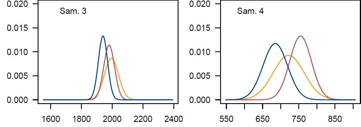
Figure 7. Distribution of conventional dates by laboratory, for samples 1 to 4.
Figure 7 shows that sample 1 has dates that only slightly overlap, unlike the other three dated samples. Starting from this first observation, we will therefore test the agreement (compatability) of the results from the different laboratories.
Are the Results from Different Laboratories in Agreement?
To answer this question, the authors of the 1988 study follow the methodology proposed by Ward and Wilson (1978). This consists of carrying out a statistical test of homogeneity whose null hypothesis (\(H_0\)) can be formulated as follows: “the dates measured by the different laboratories on the same object are equal”.
To do this, we start by calculating the average date of each object (\(\bar{x}\)). This corresponds to the weighted average of the dates obtained by each laboratory. The use of a weighting factor (the inverse of the variance, \(w_i = \frac{1}{\sigma_i^2}\)) makes it possible to adjust the relative contribution of each date (\(x_i\)) to the average value.
\[\bar{x} = \frac{\sum_{i=1}^{n}{w_i x_i}}{\sum_{i=1}^{n}{w_i}}\]This average date is also associated with an uncertainty (\(\sigma\)):
\[\sigma = \left(\sum_{i=1}^{n}{w_i}\right)^{-1/2}\]From this average value, we can calculate a statistical test variable (\(T\)) allowing the comparison of the measured ages to a theoretical date (here the average date) for each dated object.
\[T = \sum_{i=1}^{n}{\left( \frac{x_i - \bar{x}}{\sigma_i} \right)^2}\]\(T\) is a random variable which follows a \(\chi^2\) law with \(n-1\) degrees of freedom (\(n\) is the number of datings per object, here \(n = 3\) for the 3 labs). From \(T\), it is possible to calculate the \(p\) value, that is to say the risk of rejecting the null hypothesis even though it is true. By comparing the \(p\) value to a threshold \(\alpha\) fixed in advance, we can determine whether or not it is possible to reject \(H_0\) (if \(p\) is greater than \(\alpha\), then we cannot reject the null hypothesis). Here we set this \(\alpha\) value to 0.05. We therefore estimate that a 5% risk of making a mistake is acceptable.
The following code allows you to calculate for each sample, its average date, the associated uncertainty, the \(T\) statistic and the \(p\)-value.
## Create a data.frame to collect the results
## Each line corresponds to a sample.
## The columns correspond to:
## - average age
## - uncertainties associated with that age
## - the homogeneity test statistic
## - p-value of the homogeneity test
dates <- as.data.frame(matrix(nrow = 4, ncol = 4))
rownames(dates) <- paste("Sam.", 1:4, sep = " ")
colnames(dates) <- c("age", "uncertainties", "chi2", "p")

## For each dated object:
for (j in 1:ncol(turin)) {
  age <- turin[, j, 1] # extract the dates
  inc <- turin[, j, 2] # extract the uncertaintites

  # calculate the weighted average
  w <- 1 / inc^2 # Weighting factor
  moy <- stats::weighted.mean(x = age, w = w)

  # calculate the uncertainty associated with the weighted average
  err <- sum(1 / inc^2)^(-1 / 2)

  # calculate the test statistic
  chi2 <- sum(((age - moy) / inc)^2)

  # calculate the p value
  p <- 1 - pchisq(chi2, df = 2)

  # collect the results
  dates[j, ] <- c(moy, err, chi2, p)
}

dates
##              age   uncert      chi2          p
## Sam. 1  689.1192 16.03791 6.3518295 0.04175589
## Sam. 2  937.2838 15.85498 0.1375815 0.93352200
## Sam. 3 1964.4353 20.41230 1.3026835 0.52134579
## Sam. 4  723.8513 19.93236 2.3856294 0.30336618
We see that sample 1 has a \(p\)-value of 0.04. As this is lower than the threshold \(\alpha\) set, hypothesis \(H_0\) can be rejected. This means that the differences observed between the dates obtained in this sample are significant. The \(p\) values obtained for the other samples are respectively 0.92, 0.52 and 0.30: hypothesis \(H_0\) cannot therefore be rejected in these cases.
This fluctuation in the dates of sample 1 is probably linked to heterogeneity of the measurements within one of the laboratories.14
Date Calibration
In accordance with the results of the previous tests, the different dates obtained for sample 1 will be calibrated separately, while we will be able to calibrate the average dates of samples 2, 3 and 4. The calibration is carried out with the calibrate() function of the rcarbon package. We can then use summary() to obtain a summary of the calibrated dates. By default, summary() displays dates in calendar years BP.
## load the rcarbon package
library(rcarbon)

## calibrate dates for sample 1
dates_sam1 <- calibrate(
  x = turin[, 1, 1],
  errors = turin[, 1, 2],
  ids = rownames(turin),
  calCurves = "intcal20",
  verbose = FALSE
)

## display the ages calibrated to 95%
summary(dates_sam1, prob = 0.95)
##    DateID MedianBP p_0.95_BP_1 p_0.95_BP_2
## 1 Arizona      600  667 to 623  612 to 555
## 2  Oxford      682  725 to 660    NA to NA
## 3  Zurich      648  671 to 633  589 to 563
## calibrate the average ages of samples 2, 3 and 4
datess_sam234 <- calibrate(
  x = dates$age[-1],
  errors = dates$uncertainties[-1],
  ids = rownames(dates)[-1],
  calCurves = "intcal20",
  verbose = FALSE
)

## display the ages calibrated to 95%
summary(datess_sam234, prob = 0.95)
##DateID MedianBP  p_0.95_BP_1  p_0.95_BP_2
##1 Sam. 2      850   910 to 841   837 to 792
##2 Sam. 3     1893 1974 to 1966 1943 to 1829
##3 Sam. 4      670   682 to 653     NA to NA
Some of the dates calibrated at 95% belong to the union of several HPD intervals. The hpdi() function allows you to calculate the HPD intervals for each calibrated date (note, hpdi() returns ages expressed in cal years BP) and the probability associated with each interval:
## HPD intervals at 95% of sample 1 ages
(hpd_sam1 <- hpdi(dates_sam1, credMass = 0.95))
## [[1]]
##      startCalBP endCalBP      prob
## [1,]        667      623 0.4298236
## [2,]        612      555 0.5305958
##
## [[2]]
##      startCalBP endCalBP      prob
## [1,]        725      660 0.9505207
##
## [[3]]
##      startCalBP endCalBP      prob
## [1,]        671      633 0.5776311
## [2,]        589      563 0.3795208
## HPD intervals at 95% of sample ages 2, 3 and 4
(hpd_sam234 <- hpdi(datess_sam234, credMass = 0.95))
## [[1]]
##      startCalBP endCalBP      prob
## [1,]        910      841 0.5442044
## [2,]        837      792 0.4058215
##
## [[2]]
##      startCalBP endCalBP       prob
## [1,]       1974     1966 0.02250843
## [2,]       1943     1829 0.93019646
##
## [[3]]
##      startCalBP endCalBP      prob
## [1,]        682      653 0.9534739
How to Interpret these Dates
We are first interested in control samples 2, 3 and 4. The distributions of conventional (y-axis) and calendar (x-axis) dates can be represented with the calibration curve using the plot() function. Figure 8 then shows that their calibrated dates are in agreement with the dating known elsewhere.
par(mfrow = c(1, 3), mar = c(4, 1, 3, 1) + 0.1, las = 1)

## For samples 2, 3, and 4:
for (i in 1:3) {
  plot(
    x = datess_sam234,
    ind = i,
    HPD = TRUE,
    credMass = 0.95,
    calendar = "BCAD",
    xlab = "Years BC/AD",
    axis4 = FALSE
  )
  mtext(text = rownames(dates)[-1][[i]], side = 3)
}
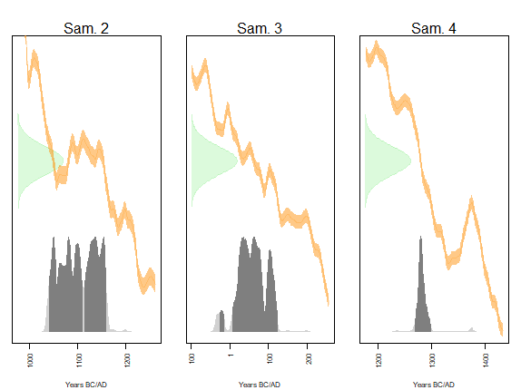
Figure 8. Distribution of conventional and calendar dates of the mean ages of samples 2, 3 and 4. The dark gray areas correspond to the 95% HPD interval. IntCal20 calibration curve.
-
The calendar date of sample 2 has a 95% chance (HPD interval) of being in the union of the intervals [1040;1109] (54%) and [1113;1158] (40%), in agreement with a dating expected around the 11th-12th centuries AD.
-
The calendar date of sample 3 has a 95% chance (HPD interval) of being in the union of the intervals [-25;-17] (2%) and [7;121] (93%), in agreement with an expected dating between -110 and 75.
-
The calendar date of sample 4 has a 95% chance (HPD interval) of being between 1267 and 1297, in agreement with an expected dating between 1290 and 1310.
The radiocarbon dates obtained by the different laboratories for sample 1 were calibrated separately. The multiplot() function makes it possible to simultaneously represent the distributions of calibrated ages (expressed in years BC/AD) for the three laboratories (fig. 9).
## set graphic parameters
par(mar = c(4, 1, 0, 1) + 0.1)

## represent the ages obtained by the three laboratories (sample 1)
multiplot(
  x = dates_sam1,
  type = "d",
  decreasing = TRUE,
  HPD = TRUE,
  credMass = 0.95,  # 95%
  calendar = "BCAD", # calendar reference
  xlab = "years AD"
)
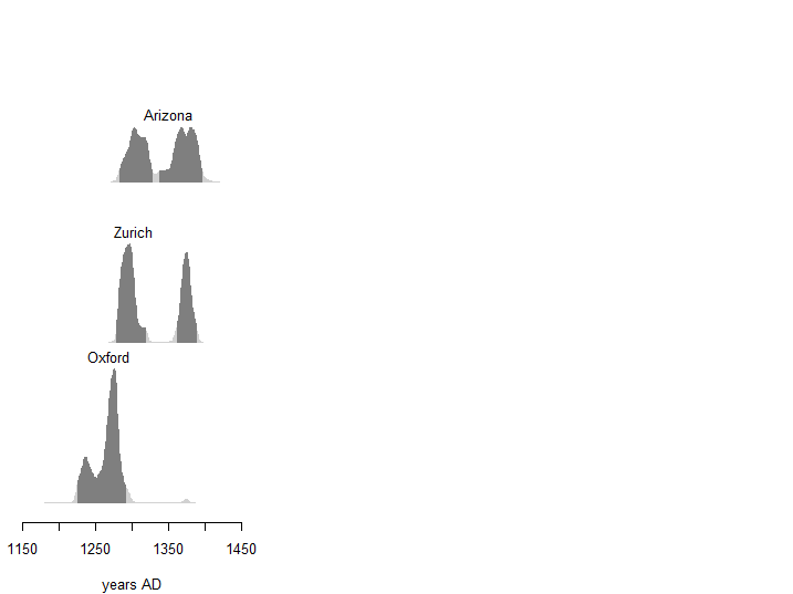
Figure 9. Distribution of calendar ages of sample 1 obtained by the different laboratories. Dark gray areas correspond to the 95% HPD interval. IntCal20 curve.
If the analysis of the conventional ages obtained by the different laboratories for sample 1 reveals a certain heterogeneity, we nevertheless note that the calibrated dates all belong to the 13th and 14th centuries. Although we cannot give a more precise interval, these results are in agreement with the appearance of the first written mentions of the Shroud and reasonably allow us to exclude the hypothesis of authenticity of the relic.
How to Present your Results
In order to publish the radiocarbon dates in rigorous manner, and to enable the results to be verified and used by others, it is a good idea to always include a certain number of information elements. For example, we can write clearly:
Sample ETH-3883 is dated at 676 ± 24 years BP, calibrated at [671;633] (58%) or [589;563] (38%) cal BP or [1279;1317] (58%) or [ 1361;1387] (38%) AD (95% HPD intervals) with IntCal20 (Reimer et al. 2020), R 4.0.3 (R Core Team, 2020) and the rcarbon 1.4.1 package (Crema and Bevan, 2020 ).
When we write our dates in this way, we have the following main points for others to read:15
- The conventional date and its uncertainty (676 ± 24 years BP), accompanied by the identification number given by the laboratory (ETH-3883);
- The calibrated date in the form of one or more intervals (due to its particular distribution, a calibrated date is always given in the form of intervals), specifying the probability associated with each interval and the temporal reference used (cal BP or BC/AD);
- The calibration curve used and the corresponding reference: IntCal20 (Reimer et al. 2020), the versions of R and the package used (R version 4.0.3 and rcarbon version 1.4.0).
Conclusion
Calibrating radiocarbon dates allows their transposition into a calendar time frame. This step is key to interpreting the results, especially since the rhythm of the carbon-14 “clock” varies over time. In this lesson, we learned how to combine conventional dates and test for consistency before calibrating them. We also saw how to graphically represent these date and how to present the results with all the information necessary for their reproduction.
Endnotes
Bibliography
Anderson, E. C., W. F. Libby, S. Weinhouse, A. F. Reid, A. D. Kirshenbaum, & A. V. Grosse. 1947. “Radiocarbon From Cosmic Radiation”. Science 105 (2735): 576‑77. https://doi.org/10.1126/science.105.2735.576.
Arnold, J. R., & W. F. Libby. 1949. “Age Determinations by Radiocarbon Content: Checks with Samples of Known Age”. Science 110 (2869): 678‑80. https://doi.org/10.1126/science.110.2869.678.
Bevan, A. & Crema, E. R. 2020. rcarbon: Methods for calibrating and analysing radiocarbon dates. Package R, v1.4.0. https://CRAN.R-project.org/package=rcarbon
Calabrisotto, C. S., Amadio, M., Fedi, M. E., Liccioli, L. & Bombardieri, L. 2017. “Strategies for Sampling Difficult Archaeological Contexts and Improving the Quality of Radiocarbon Data: The Case of Erimi Laonin Tou Porakou, Cyprus.” Radiocarbon 59 (6): 1919–30. https://doi.org/10.1017/RDC.2017.92.
Colman, S. M., K. L. Pierce, & P. W. Birkeland. 1987. “Suggested Terminology for Quaternary Dating Methods.” Quaternary Research 28 (2): 314-19. https://doi.org/10.1016/0033-5894(87)90070-6.
Crema, E. R. & Bevan, A. 2020. “Inference From Lage Sets of Radiocarbon Dates: Software and Methods”. Radiocarbon. https://doi.org/10.1017/RDC.2020.95.
Damon, P. E., D. J. Donahue, B. H. Gore, A. L. Hatheway, A. J. T. Jull, T. W. Linick, P. J. Sercel, et al. 1989. “Radiocarbon dating of the Shroud of Turin”. Nature 337 (6208): 611‑15. https://doi.org/10.1038/337611a0.
Dean, J. S. “Independent Dating in Archaeological Analysis”. In Advances in Archaeological Method and Theory, 223‑55. Elsevier, 1978. https://doi.org/10.1016/B978-0-12-003101-6.50013-5
Hyndman, R. J. 1996. “Computing and Graphing Highest Density Regions.” The American Statistician 50 (2): 120-26. https://doi.org/10.2307/2684423.
Libby, W. F. “Radiocarbon Dating”. Nobel Lecture. Stockholm, 12 December 1960. http://www.nobelprize.org/nobel_prizes/chemistry/laureates/1960/libby-lecture.html.
Millard, A. R. 2014. “Conventions for Reporting Radiocarbon Determinations.” Radiocarbon 56 (2): 555-59. https://doi.org/10.2458/56.17455.
Millot, G. Comprendre et réaliser les tests statistiques à l’aide de R - Manuel de biostatistique. Troisième édition. Louvain-la-Neuve : De Boeck, 2014.
O’Brien, M. J, & R. L. Lyman. Seriation, Stratigraphy, and Index Fossils: The Backbone of Archaeological Dating. Dordrecht : Springer, 2002.
Reimer, P. J., M. G. L. Baillie, E. Bard, A. Bayliss, J. W. Beck, P. G. Blackwell, C. Bronk Ramsey, et al. 2009. “IntCal09 and Marine09 Radiocarbon Age Calibration Curves, 0–50,000 Years Cal BP”. Radiocarbon 51 (4): 1111‑50. https://doi.org/10.1017/S0033822200034202.
Reimer, P. J., E. Bard, A. Bayliss, J. W. Beck, P. G. Blackwell, C. Bronk Ramsey, C. E. Buck, et al. 2013. “IntCal13 and Marine13 Radiocarbon Age Calibration Curves 0-50,000 Years cal BP”. Radiocarbon 55 (4): 1869‑87. https://doi.org/10.2458/azu_js_rc.55.16947.
Reimer, P. J., W. E. N. Austin, E. Bard, A. Bayliss, P. G. Blackwell, C. Bronk Ramsey, M. Butzin, et al. 2020. “The IntCal20 Northern Hemisphere Radiocarbon Age Calibration Curve (0-55 Cal KBP)”. Radiocarbon, 1‑33. https://doi.org/10.1017/RDC.2020.41.
Scott, E. M., G. T Cook, & P. Naysmith. 2007. “Error and Uncertainty in Radiocarbon Measurements”. Radiocarbon 49 (2): 427‑40. https://doi.org/10.1017/S0033822200042351.
Ward, G. K., & S. R. Wilson. 1978. “Procedures for Comparing and Combining Radiocarbon Age Determinations: A Critique”. Archaeometry 20 (1): 19‑31. https://doi.org/10.1111/j.1475-4754.1978.tb00208.x.
Walsh, B., & Schwalbe, L. 2020. “An Instructive Inter-Laboratory Comparison: The 1988 Radiocarbon Dating of the Shroud of Turin”. Journal of Archaeological Science: Reports 29: 102015. https://doi.org/10.1016/j.jasrep.2019.102015.
-
As opposed to relative dating which orders a series of events. Strictly speaking, there is no absolute dating method because they all fit into a specific frame of reference. Some authors thus prefer to speak of quantifiable dating (O’Brien and Lyman, 2002). However, for convenience, we retain this terminology here, since it is understood that an absolute date is expressed as a point on a standard scale for measuring time (Dean, 1978). ↩
-
As support for this lesson, it may be helpful to read the introductory chapters of Comprendre et réaliser les tests statistiques à l’aide de R : Manuel de Biostatistique by Gaël Millot (2014) (in French). ↩
-
Anderson et al. 1947. ↩
-
Colman, Pierce & Birkeland, 1987. ↩
-
We use the year 1950 as our reference, because it corresponded to the standard astronomical era (during these first developments of the radiocarbon method). Today we use 1950 as it also allows us to have a reference which sufficiently precedes the consequences of atmosphere nuclear tests. ↩
-
The reality is more complex, notably with the reality of isotope fractionation. ↩
-
See, for example, Calabrisotto et al. (2017). ↩
-
Arnold & Libby, 1949; Libby, 1960. ↩
-
There actually exists three series of calibration curves: IntCal for the northern hemisphere, SHCal for the southern hemisphere, and Marine for marine samples. ↩
-
At the moment of this lesson’s first publication (in French), the curve IntCal20 has just been published. Reimer et al., 2009, 2013, 2020. ↩
-
Scott, Cook & Naysmith, 2007. ↩
-
Actually, calibration by simple interception no longer needs to be used. ↩
-
Hyndman, 1996. ↩
-
The reasons of this heterogeneity are beyond the scope of this lesson. A detailed discussion is available in the literature, see for example Walsh and Schwalbe (2020). ↩
-
Millard, 2014. ↩