This is the draft website for Programming Historian lessons under review. Do not link to these pages.
For the published site, go to https://programminghistorian.org
Contents
- Overview
- Lesson Goals Summarized
- Technical Requirements
- Part 1: Introduction to Simulations and Agent-based Modeling
- Part 2: Programming Agent-based Models with Mesa
- Part 3: A Summary, Open Questions and Next Steps
- Endnotes
Overview
In this lesson, we will provide an introduction to the simulation method of Agent-based Modeling (often abbreviated ABM) via an Agent-based Model of a historical letter sending network, implemented with the python-package mesa.
The historical case that inspires this lesson is the Republic of Letters, an early modern network of scholars who wrote each other extensively, thereby fertilizing each others thinking, which has been extensively studied with digital methods1,2. With our model, we want to better understand the social dynamics of these correspondence networks and how they were able to shape the scientific thought of the time.
The model we are building together will be relatively basic and will only feature simple interactions like sending letters. Those simple interactions will lead to correspondence networks that are structurally similar to those observed in actual, historical data-sets on letter sending.
The model we build here will not be sufficiently complex to give genuinely valuable perspectives on this case study on its own, but it will highlight some key properties of Agent-based Modeling and ways to implement them. Crucially, by the end of this lesson, you will be able to extend the model further with more complex functionalities.
In the first part, you will learn what historical simulation methods are all about, their methodological and epistemological quirks, and how to start applying Agent-based Modeling to your research.
In the second part, you can follow a step-by-step guide to build your first Agent-based Model with mesa. This will be accompanied by further comments and reflections on the methodology of Agent-based Modeling.
In the third part, we will tell you about ways to extend the model and further enhance your expertise in building Agent-based Models.
Lesson Goals Summarized
This lesson intends to:
- teach conceptual basics of simulation methods and ‘Agent-based Modeling’ for historians,
- teach fundamentals of the python-package
mesafor programming Agent-based Modeling, - give you guidance and resources for extending your Agent-based Modeling knowledge beyond this tutorial, as well as
- give an overview over methodological and epistemological caveats, challenges, and things to think about when programming your own historical Agent-based Models.
Users of different skill levels and interests will find this lesson useful, for example if:
- you are completely unfamiliar with simulation methods and Agent-based Modeling and want a thorough introduction,
- you already know about Agent-based Modeling conceptually and are wondering whether it can be useful for your own research project,
- you already know that Agent-based Modeling might be useful for your research and now want to learn about how the process of modeling and technical implementation of an Agent-based Modeling can work,
- you are familiar with all of the above and need a starting point for implementing Agent-based Models with
mesa.
Technical Requirements
Note that a solid understanding of Python is required for this lesson! If you are unfamilliar with features of python such as ‘classes’ but do have previous python experience, you could head over to w3schools to get up to speed.
For this lesson, mesa and its dependencies are necessary. Additionally we will use matplotlib for visualizations and numpy for some calculations.
Execute the code block below in a command line (or in a jupyter-notebook) to install mesa and its dependencies. If you want to follow through the tutorial on your local machine, you need to set up an environment with mesa installed. If you do not know how to do this, we have a simple step-by-step instruction, which we compiled for a workshop.
Setup an environment:
If you already have Python (version >=3.9) installed, running the following code in a terminal should give you a new virtual environment with the mesa package:
python3 -m venv env
source env/bin/activate
pip install mesa
If you would like to have a more gentle and comprehensive introduction, head over to the tutorial introducing Python.
try:
  import mesa
except:
  !pip install mesa
Part 1: Introduction to Simulations and Agent-based Modeling
1.1 Why use Historical Simulations for our case study?
In this lesson, we are motivated by trying to better understand the social dynamics that might have shaped intellectual networks in the past, specifically during the early modern period. In this time in Europe, a primarily letter-based network of scholars of different nationalities emerged, often referred to as the ‘Republic of Letters’. The effect of this network on the history of science in Europe and the world is deemed to be pivotal3, but beyond studying the shape of the networks and speculating about the historical sources we have, it is hard to understand why and how these networks came to the shape we observe today.
Questions related to this are usually hard to answer in a systematic and methodologically sound way. Consider for example the following questions: Which social and intellectual dynamics led to some people being central in the network? How did people form and develop their connections in the network? What effect did simple limiting elements such as distance, infrastructure and technology have on the shape of the network?
We can pose some limited hypotheses regarding those questions and might draw on network research for the sources for some hints and correlations, but it is hard to reliably test those hypotheses.
One of the main motivations for using historical simulation, or even simulations in general, is precisely this: operationalizing hypotheses about the underlying reasons for (historical) phenomena, comparing them against what we observe in “reality”. That way, we can test if our hypotheses can explain these phenomena.
We could for example assume that, in a particular historical letter network, more famous people receive a higher amount of letters, and that this effect gets stronger over time by being self-reinforcing. Or, we could consider it more likely that a person will send a letter to someone who is a rather close neighbor compared to someone far away. Another area of hypotheses arises if we consider the topic of a letter as well. Letters could more likely be sent if a sender agrees with a receivers personal opinion, but it could also be the opposite.
Building a simulation model of this letter network would allow us to represent different hypotheses about its dynamics and might help us gain a more thorough understanding of its workings. But what does it actually mean to build a simulation?
1.2. What are Simulations?
To start of with, we want to give you a very general definition of the term ‘simulation’, before we dive into what this actually means:
“The term ‘simulation’ describes a number of different methods of model-based, experimental reproduction of a real-world or hypothetical process or system4.”
As the definition says, the basis of every simulation is an executable simulation model. This is a class of models - similar to data models - that can be expressed conceptually (i.e., with more or less stringent language), logically (i.e., in logical terms of ‘if-then’ ‘is/is not’ etc.) or mathematically (i.e., through mathematical terms). To execute a simulation model, however, it must be formalized, i.e., converted into computer-readable form. Just like what we would do in a data model, in a simulation model we formally describe our ideas of a person, place, or the event of a letter exchange, but additionally, we also describe triggers for certain actions, movements, and interaction rules.
We can then run this model, the actual simulation, to see how these rules, attributes, decisions, etc. in our letter exchange model play out together over time. Once we observed these new pieces of information - essentially the model outputs - of our simulation run, our model can be revised and then run again. The process of building a simulation model is constantly cycling between phases of running the model, interpreting the results, and then adapting the model for further experiments. In this sense, simulation methodology is comparable to the hermeneutic circle of heuristics, critique, and interpretation historians are used to5.
Now to the last part of the definition regarding real-world or hypothetical subject matters. Many historians probably hold a cautious view of the nature of historical reality and - more importantly - our ability as scholars to describe it. Just as sources are king in traditional history, data is queen in Digital History.
However, as we already tried to hint at, the objects of the simulation are not data alone, but our hypotheses about history, i.e. all the assumptions we have about the past that we believe connect our data into a plausible narrative. By building a historical simulation model we are automatically moving ‘from the actual to the possible’6.
The alluring but at the same time tricky opportunity of historical simulations therefore is to go between and beyond the actual data we have at our disposal in a formalized way. One crucial difference here to epistemologically similar, traditional counterfactual approaches to history is the formalized, systematic and experimental nature of simulations.
There is also one last important caveat left to be mentioned about definitions of simulation methods: there are a lot, and especially in history the discussion about which is the most suitable is in progress! Definitions sometimes depend more on what its goals are (e.g., educational or scientific, see note below), sometimes they try to exclude certain applications of simulations from its definition to avoid some of the epistemological challenges posed by simulations for historical studies [see Scheuermann^7a]. We have opted to present you one of the more open and general definitions of simulation, for clarity’s sake and to avoid the epistemological controversies connected to some of those definitions. In short, we do believe that ‘simulation’ is a good general term for the method we are presenting here.
Note: So far, we talked about historical simulations as analytical tools for researching history, and this will remain our focus in this lesson. However, simulations can also be didactic tools for interactive and immersive teaching, they are sometimes a synonym for more static 3D reconstructions which are used to visualise past spaces7, and they are themselves the subject of research8.
Now that you have a general idea of what historical simulations are about theoretically, we need to dive into what a good methodological approach for our case study is. We want to model the interactions of individuals - the people sending letters to each other. Thus, we need a modeling approach that emphasizes those one-on-one interactions: a so called Agent-based Model.
1.3: What is Agent-based Modeling?
Agent-based modeling (sometimes ABM for short) is a simulation method where relations and interactions of individual entities, for example humans, organizations, items, etc., with each other and with their environment are simulated9.
Ideally, these interactions make some emergent patterns appear, meaning they are not prescribed in the simulation by the researcher, but dynamically arise out of the system. In our case, for example, we actively do not want to prescribe in the model how the letter network should look in the end. We would like to see what shapes of the letter networks emerge dynamically from the letter-sending rules we have set up. If the shape differs wildly from what we observe in our data, we know we are probably way off with our hypotheses (or the way we formalized them).
Agent-based Models are especially suited to allow for those emergent processes to appear. In general, emergent phenomena in human activity and behavior pose a number of questions that are of central interest for and feature much in debates among historians, such as: How and why did a society change? Why did some states get the upper hand over others in some time frame? How did some new technology or idea spread from one group of people to another?
These questions, it has to be stressed, are different from those we might have about specific individuals. For our case, for example, we would not be able to ask “Why did Christiaan Huygens send this particular letter to Johannes Hevelius?”, but rather “Is there a reason and pattern in intellectuals of that era sending each other letters?”.
As a simulation method, Agent-based Modeling offers the opportunity to formally and systematically pursue these kinds of questions by building models of the pertaining case study and experiment with that model.
To summarize, the goal of this method is to link the emergent patterns and phenomena at the systemic macro-level with the individual micro-level behavior of interacting entities, the name-giving “Agents”. The focus is often the patterns and underlying dynamics in history rather than any unique case on its own.
1.4: Historical Context of Agent-based Modeling
Simulations were among the first digital methods applied in historical research. Some of the earlier historical simulations were done by prominent figures of the early digital humanities and digital history, such as Michael Levison10 or Peter Laslett from the Cambridge Group for the History of Population and Social Structure11. The latter also coined this simulative approach to “experimental history”, to underline the experimental and iterative nature of the process12.
Agent-based Modeling as a term for the kind of simulation approach we just described was coined during the 1990s, pioneered among others by Joshua M. Epstein and Robert Axtell13.
Similar, individual-based simulation approaches have existed from at least the 1960s, though. Tim Gooding puts the origins of Agent-based Modeling at 1933, when Enrico Fermi first used the so-called Monte-Carlo-Method with mechanical computing machines14. Another early example includes the aforementioned Peter Laslett, who, together with Anthropologist Eugene Hammel and Computer scientist Kenneth W. Wachter, devised individual-based Monte-Carlo Simulations on household structures in early modern England11.
Since then, a number of changes occured that warrant a distinction between those efforts and the newer, actual Agent-based Models. For one, changes in hardware, software and programming paradigms have led to a much higher performance and affordability of bigger and more complex models. Also, the epistemological framework of emergent properties in systems we described in Sec. 1.2 is heavily inspired by modern thinking on Complex Adaptive Systems, which itself has roots into the 1950s and before, but is mainly a product of recent scholarly activity15. In the newer Agent-based Modeling, there is a bigger principle emphasis on the relevance of heterogenuous agents, processes of social learning, coupling of micro- and macro-level phenomena and on theory-agnosticism.
Today, Agent-based Modeling and simulations in general are starting to appear more frequently in historical research, most notably in Archaeology16, but in the context of Digital History17 and Digital Humanities6 as well.
Part 2: Programming Agent-based Models with Mesa
In this chapter, we will start to actually implement a simple simulation model of early modern letter exchange using the python package mesa. Before we start, we will reiterate our exact goals for this model, which will guide the process of building it. We then proceed to clarify some key concepts of Agent-based Models that might be unclear to a newcomer to the method.
2.1 Goals
In this lesson, we want to model the networks of letter exchange of scholars in and around the 17th century often referred to as Republic of Letters. For the purposes of this, a very basic model suffices, but there are some aspects we need at the very least to approach an actual model of the Republic of Letters.
We want to have:
- a space in which the scholars are situated and can move,
- a number of scholars ‘living’ and moving in that space,
- the ability of scholars to send each other letters,
- the ability of the scholar in front of the screen - that’s you! - to read and interpret the simulation run.
You might already think of ways in which this simple shopping list for our lesson model would not be adequately representing the Republic of Letters. As we mentioned, the result of this lesson will not yet be a plausible model, but perhaps the start of one. We will give you some ideas of how to extend the model and make it more historically plausible at the end.
2.2 What about Data?
You might ask yourself where actual data comes into the mix. One peculiar thing about simulations is, that not everything and sometimes even nothing in a simulation model is based 1-to-1 on quantitative data. This is because with simulations, ‘we are not trying to model the world […] [w]e are trying to model ideas about the world.’18.
Data is very important for historical simulations, too, but the role it plays is different to, say, network analysis, where data is the whole basis of a network in the first place.
In historical simulations such as ours here, we could use data for different things. We could use data on historical people of the Republic of Letters to inform the building of our agents. We can use surviving data on the historical network to compare them to the results of our simulation in order to see how much the latter deviates from the historical data. We could (and should) also use extended domain knowledge - be it quantitative data or qualitative scholarship - to make the properties of our agents, the decisions they can make and the environment they move in more historically plausible.
At the stage of this simple initial model, we actually don’t need any data. For our own project, which essentially is a more complicated version of this model, we do use a dataset which you can read more about in the documentation of the model we build in our research. At the end of the lesson, we will also go into more depth about the methodological implications this has for historical research.
2.3 Key concepts of Agent-based Models
Before we finally start coding, a last couple of remarks have to be made about key concepts in Agent-based Modeling that will reappear in the rest of this chapter in a practical way.
Agents
We already mentioned agents a lot - it’s in the name, after all! Agents are any entity in the model that can act: it can move, alter properties of itself, other agents or its environment. Agents do not have to be humans. According to the very wide conception of acting here, also animals, plants, organizations or even objects can be Agents within the logic of the model.
Space and Environment
Those two concepts are sometimes used interchangably, but they are usually the, at least, second most important feature of an Agent-based Model. This is not only the dimensional space in which Agents can move, but also maybe filled with more static elements of the model (such as climate, or certain natural features). But space can also be understood very abstractly - for example, in a different model we built at ModelSEN, the space agents ‘move’ in is a representation of the knowledge they hold.
Model
We also already mentioned that a model and the process of modeling in Agent-based Modeling is somewhat different than in other types of models. The model is the collection of agents and environment, but also their interactions and any other logics that tie everything together. The model is really only complete when it is running, which means all the interactions of agents and environment are computed.
Time
That of course means that each model needs to have a formal concept of how these steps are computed, or in other words: a concept of time. There are different ways to model the passage of time in an Agent-based Model, sometimes in discrete time steps (kind of like turns in a game), sometimes in a more continuous flow of time.
Experimentation
The temporal nature of simulation models also means that you will have to run and tweak your model all the time. This practice of iteration and experimentation is not just a practical necessity, though, but in many ways a virtue of the method. We already likened that process to the hermeneutical circle. Similarly, here, your knowledge of the dynamics of the system, specifically what can and cannot work within the bounds of your assumptions, is growing over time. One important implication of this is that any simulation model provides at most an imperfect perspective on history.
2.4 Overview of Mesa
In this tutorial we will make use of mesa, an open-source Agent-based Modeling framework written in Python. Mesa offers predefined functions to implement the key ingredients of an Agent-based Modeling. The package is in development since 2015 and has aquired a large community of users and contributors (see the mesa Github repository). Its relative longevity and popularity makes it a good choice to start using Agent-based Modeling.
If you are more familiar with other programming languages, you can consider applying the ideas of this tutorial, e.g., in the frameworks NetLogo (a dedicated Agent-based Modeling language) or MASON (based on Java).
In mesa a minimal Agent-based Modeling implementation consists of a definition of an “agent” class and a “model” class. The “model” class holds the model-level attributes (for example attributes of the environment or other external factors), manages the agents, and generally handles the global processing level of our model.
Each instantiation of the model class will be a specific model run. Each model will contain multiple agents, all of which are instantiations of the agent class. Both the model and agent classes are child classes of mesa’s generic Model and Agent classes. In line with the above introduced idea of individual-based modeling, each agent should have a unique id to allow tracking during the simulation.
Another important aspect of mesa is the scheduler. The scheduler keeps track of which agent should act when. This process is called “activation” in the terms of mesa, and there are a number of predifined activation procedures: random, simultaneous, or staged activation. For this tutorial we will make use of random activation, meaning that all agents act one after another, but the order is random at each new step of the model.
Some research questions might require the agents to interact in/with a space. This could be a geographical space or something more abstract. Sometimes, like in this tutorial, a simple abstracted representation of relative distance is sufficient, for example in form of a two-dimensional grid. Mesa also supports hexagonal, continuous or network grids, which are useful for e.g. covering a geographical space or simulating social relations. If a simulation relies on geographical map projections, an additional package from the mesa project might be useful: mesa-geo.
2.5 Building the Model
We are now ready to start with the actual modelling. For this we first introduce the agents, then a model, and then the activation of these agents. Let’s get started!
"""To start with, let's import the mesa module"""
import mesa
2.5.1 Setting up the model
To begin writing the model code, we start with two core classes: one for the overall model, the other for the agents.
Let’s start with the new agent class: class LetterAgent(mesa.Agent).
For now, each agent has only two variables: how much letters it currently has sent and received. Each agent will also have a unique identifier (i.e., a name), stored in the unique_id variable. Giving each agent a unique id is a good practice when doing agent-based modeling.
class LetterAgent(mesa.Agent):
    """An agent with no initial letters."""

    def __init__(self, unique_id, model):
        super().__init__(unique_id, model)
        self.letters_sent = 0
        self.letters_received = 0
Next, we need to have a model: class LetterModel(mesa.Model). There is only one model-level parameter: how many agents the model contains. When a new model is started, we want it to populate itself with the given amount of agents.
class LetterModel(mesa.Model):
    """A model with N agents."""

    def __init__(self, N):
        super().__init__()
        self.num_agents = N
        # Create N number of agents
        for i in range(self.num_agents):
            a = LetterAgent(i, self)
2.5.2 Adding time
Time in most agent-based models moves in steps, sometimes also called ticks. At each step of the model, one or more of the agents – usually all of them – are activated and take their own step, changing internally and/or interacting with one another or the environment.
The scheduler is a special model component which controls the order in which agents are activated. For example, all the agents may activate in the same order every step, their order might be shuffled, we may try to simulate all the agents acting at the same time, and more. Mesa offers a few different built-in scheduler classes, with a common interface. That makes it easy to change the activation regime a given model uses, and see whether it changes the model behavior. This may not seem important, but scheduling patterns can have an impact on your results19.
For now, let’s use one of the simplest ones: RandomActivation20, which activates all the agents once per step, in random order.
self.schedule = mesa.time.RandomActivation(self)
Every agent is expected to have a step method. The step method is the action the agent takes when it is activated by the model schedule. We add an agent to the schedule using the add method; when we call the schedule’s step method, the model shuffles the order of the agents, then activates and executes each agent’s step method.
def step(self):
    # The agent's step will go here.
    # For demonstration purposes we will print the agent's unique_id
    print("Hi, I am agent " + str(self.unique_id) + ".")
Adding all parts together, the model code with the scheduler added looks like this.
class LetterAgent(mesa.Agent):
    """An agent with no initial letters."""

    def __init__(self, unique_id, model):
        super().__init__(unique_id, model)
        self.letters_sent = 0
        self.letters_received = 0

    def step(self):
        # The agent's step will go here.
        # For demonstration purposes we will print the agent's unique_id
        print("Hi, I am agent " + str(self.unique_id) + ".")

class LetterModel(mesa.Model):
    """A model with N agents."""

    def __init__(self, N):
        super().__init__()
        self.num_agents = N
        self.schedule = mesa.time.RandomActivation(self)
        # Create N number of agents
        for i in range(self.num_agents):
            a = LetterAgent(i, self)
            self.schedule.add(a)

    def step(self):
        """Advance the model by one step."""
        self.schedule.step()
At this point, we have a model which runs – it just doesn’t do anything. You can see for yourself with a few easy lines:
empty_model = LetterModel(10) # create a model with 10 agents
empty_model.step() # execute the step function once
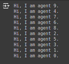
Figure 1. Currently, the only thing our agents do is say Hi!
Bonus Question 1: Try changing the scheduler from RandomActivation to BaseScheduler. What do you observe at the agents output? What would be necessary in the definiton of the agents if you would like to use StagedActivation? Hint: Have a look in the source code of
mesa.time!
2.5.3 Agent Step
Now we just need to have the agents do what we intend them to do: send each other letters.
To allow the agent to choose another agent at random, we use the model.random random-number generator. This works just like Python’s random module, but with a fixed seed set when the model is instantiated. This can be used to later replicate a specific model run.
To pick an agent at random, we need a list of all agents. Notice that there isn’t such a list explicitly in the model. The scheduler, however, does have an internal list of all the agents it is scheduled to activate.
With that in mind, we rewrite the agent step method like this:
class LetterAgent(mesa.Agent):
    """An agent with no initial letters."""

    def __init__(self, unique_id, model):
        super().__init__(unique_id, model)
        self.letters_sent = 0
        self.letters_received = 0

    def step(self):
        other_agent = self.random.choice(self.model.schedule.agents)
        other_agent.letters_received += 1
        self.letters_sent += 1
2.5.4 Running your first model
With that last piece in hand, it’s time for the first rudimentary run of the model. Let’s create a model with 10 agents, and run it for 20 steps.
model = LetterModel(10)
for i in range(20):
    model.step()
Next, we need to get some data out of the model.
Specifically, we want to see how many letters each agent sent or received. We can get the values with list comprehension, and then use matplotlib (or another graphics library) to visualize the data in a histogram.
import matplotlib.pyplot as plt
agent_letters_recd = [b.letters_received for b in model.schedule.agents]
plt.hist(agent_letters_recd)
plt.show()
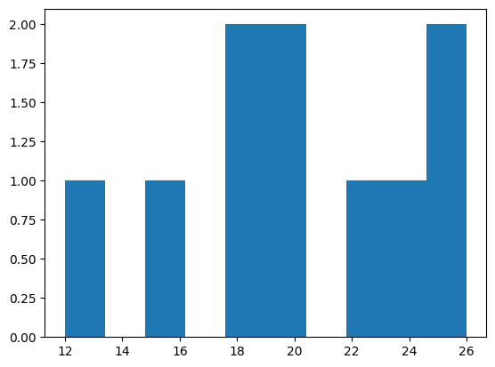
Figure 2. Histogram of the letters received by all agents
You should see something like the distribution above. Yours will almost certainly look at least slightly different, since each run of the model is random and unique, after all.
To get a better idea of how a model behaves, we can create multiple model runs and see the distribution that emerges from all of them. We can do this with a nested for loop:
all_letters_rec = []

# This runs the model with 10 agents 100 times, each model executing 10 steps.
for j in range(100):
    # Run the model
    model = LetterModel(10)
    for i in range(10):
        model.step()

    # Store the results
    for agent in model.schedule.agents:
        all_letters_rec.append(agent.letters_received)


plt.hist(all_letters_rec, bins=range(max(all_letters_rec) + 1))

plt.show()
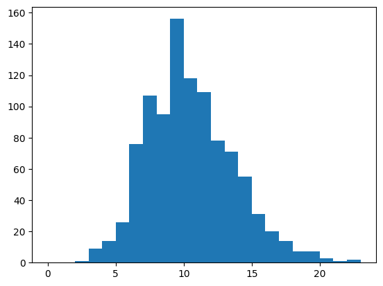
Figure 3. Histogram of the letters received by all agents after 100 model runs
This runs 100 instantiations of the model, and runs each for 10 steps. (Notice that we set the histogram bins to be integers, since agents can only have whole numbers of letters). By running the model 100 times, we smooth out some of the ‘noise’ of randomness, and get to the model’s overall expected behavior.
For now, the letter distribution looks close to a normal distribution, or Bell curve, which is expected since the process is random. Let’s add some more comparably realistic behavior by introducing space between the agents and let that influence the letter sending decision.
Bonus question 2: Can you rewrite the above function to plot the number of sent letters? What histogram do you expect for that? Hint: Are agents sending letters in every round?
2.5.5 Adding space
Many ABMs have a spatial element, with agents moving around and interacting with neighbors. Mesa currently supports two overall kinds of spaces:
grid, and continuous. Grids are divided into cells, and agents can only be on a particular cell, like pieces on a chess board. Continuous space, in contrast, allows agents to have any arbitrary position. Both grids and continuous spaces are frequently toroidal, meaning that the edges of this ‘world’ wrap around, with cells on the right edge connected to those on the left edge, and the top to the bottom. This prevents some cells having fewer neighbors than others, or agents being able to go off the edge of the environment.
Let’s add a simple spatial element to our model by putting our agents on a grid and make them walk around at random. Instead of sending a letter to any random agent, they’ll give it to an agent on the same cell. We could imagine that this represents them being close enough to know of one another and have reason to send a letter in the first place.
Mesa has two main types of grids: SingleGrid and MultiGrid21. SingleGrid enforces at most one agent per cell; MultiGrid allows multiple agents to be in the same cell. Since we want agents to be able to share a cell, we use MultiGrid.
self.grid = mesa.space.MultiGrid(width, height, True)
We instantiate a grid with width and height parameters (in this case as integers), and a boolean as to whether the grid is toroidal. Let’s make width and height model parameters, in addition to the amount of agents, and have the grid always be toroidal. We can place agents on a grid with the grid’s place_agent method, which takes an agent and an (x, y) tuple of the coordinates to place the agent.
self.grid.place_agent(a, (x, y))
Adding all the pieces looks like this:
class LetterModel(mesa.Model):
    """A model with a certain number of agents."""

    def __init__(self, N, width, height):
        super().__init__()
        self.num_agents = N
        self.grid = mesa.space.MultiGrid(width, height, True)
        self.schedule = mesa.time.RandomActivation(self)

        # Create agents
        for i in range(self.num_agents):
            a = LetterAgent(i, self)
            self.schedule.add(a)

            # Add the agent to a random grid cell
            x = self.random.randrange(self.grid.width)
            y = self.random.randrange(self.grid.height)
            self.grid.place_agent(a, (x, y))
Under the hood, each agent’s position is stored in two ways: the agent is contained in the grid in the cell it is currently in, and the agent has a pos variable with an (x, y) coordinate tuple. The place_agent method adds the coordinate to the agent automatically.
Now we need to add to the agents’ behaviors, letting them move around and only send letters to other agents in the same cell.
First, let’s handle movement, and have the agents move to a neighboring cell. The grid object provides a move_agent method, which, like you would imagine, moves an agent to a given cell. That still leaves us to get the possible neighboring cells to move to. There are a couple ways to do this. One is to use the current coordinates, and loop over all coordinates +/- 1 away from it. For example:
neighbors = []
x, y = self.pos
for dx in [-1, 0, 1]:
    for dy in [-1, 0, 1]:
        neighbors.append((x+dx, y+dy))
But there’s an even simpler way, using the grid’s built-in get_neighborhood method, which returns all the neighbors of a given cell. This method can get two types of cell neighborhoods: Von Neumann (only includes the 4 top, bottom, left and right neighboring squares) and Moore (includes all 8 surrounding squares). It also needs an argument as to whether to include the center cell itself as one of the neighbors.
With that in mind, the agent’s move method looks like this:
class LetterAgent(mesa.Agent):
   #...
    def move(self):
        possible_steps = self.model.grid.get_neighborhood(
            self.pos,
            moore=True,
            include_center=False)
        new_position = self.random.choice(possible_steps)
        self.model.grid.move_agent(self, new_position)
Next, we need to get all the other agents present in a cell, and sent one of them a letter. We can get the contents of one or more cells using the grid’s get_cell_list_contents method, or by accessing a cell directly. The method accepts a list of cell coordinate tuples, or a single tuple if we only care about one cell.
class LetterAgent(mesa.Agent):
    #...
    def send_letter(self):
        cellmates = self.model.grid.get_cell_list_contents([self.pos])
        if len(cellmates) > 1:
            other = self.random.choice(cellmates)
            other.letters_received += 1
            self.letters_sent += 1
And with those two methods, the agent’s step method becomes:
class LetterAgent(mesa.Agent):
    # ...
    def step(self):
        self.move()
        self.send_letter()
Now, putting that all together should look like this:
class LetterAgent(mesa.Agent):
    """An agent with letters sent and received.

    The agent can move to agents in other grid cells
    and send letters to agents in the same grid cell.
    """

    def __init__(self, unique_id, model):
        super().__init__(unique_id, model)
        self.letters_sent = 0
        self.letters_received = 0

    def move(self):
        possible_steps = self.model.grid.get_neighborhood(
            self.pos, moore=True, include_center=False
        )
        new_position = self.random.choice(possible_steps)
        self.model.grid.move_agent(self, new_position)

    def send_letter(self):
        cellmates = self.model.grid.get_cell_list_contents([self.pos])
        if len(cellmates) > 1:
            other_agent = self.random.choice(cellmates)
            other_agent.letters_received += 1
            self.letters_sent += 1

    def step(self):
        self.move()
        self.send_letter()
Let’s create a model with 50 agents on a 10x10 grid, and run it for 20 steps.
model = LetterModel(50, 10, 10)
for i in range(20):
    model.step()
Now let’s use matplotlib and numpy to visualize how many agents reside in each cell. To do that, we create a numpy array of the same size as the grid, filled with zeros. Then we use the grid object’s coord_iter() feature, which lets us loop over every cell in the grid, giving us each cell’s coordinates and contents in turn.
import numpy as np

agent_counts = np.zeros((model.grid.width, model.grid.height))
for cell in model.grid.coord_iter():
    cell_content, coord = cell
    x, y = coord
    agent_count = len(cell_content)
    agent_counts[x][y] = agent_count
plt.imshow(agent_counts, interpolation="nearest")
plt.colorbar()
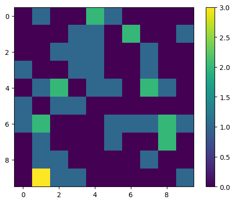
Figure 4. A colormesh showing how many agents are present on each cell of our grid space
Bonus question 3: Letters are send to direct neighbours. How could you implement sending letters only to agents far apart, e.g. with at least a distance of three cells? Hint: You will have to define a distance measure on grids, see e.g. this tutorial on similarity measures.
2.5.6 Collecting Data
So far, at the end of every model run, we’ve had to go and write our own code to get the data out of the model. This has two problems: it isn’t very efficient, and it only gives us end results. If we wanted to know the letter counts of each agent at each step, we’d have to add that to the loop of executing steps, and figure out some way to store the data.
Since one of the main goals of Agent-based modeling is generating data for analysis, mesa provides a class which can handle data collection and storage for us and make it easier to analyze.
The data collector stores three categories of data: model-level variables, agent-level variables, and tables (which are a catch-all for everything else). Model- and agent-level variables are added to the data collector along with a function for collecting them. Model-level collection functions take a model object as an input, while agent-level collection functions take an agent object as an input.
When the data collector’s collect method is called, with a model object as its argument, it applies each model-level collection function to the model, and stores the results in a dictionary, associating the current value with the current step of the model. If the input model is an Agent, the method associates the resulting value with the agent’s unique_id as well.
Let’s add a DataCollector to the model with mesa.DataCollector, and collect two variables at the agent level. We want to collect every agent’s letters sent and letters received at every step.
self.datacollector = mesa.DataCollector(
    agent_reporters={
      "Letters_sent": "letters_sent",
      "Letters_received": "letters_received"
    },
    model_reporters={
      "All letters":compute_received_letters
    }
)
Additionally, we define a new function to collect data on the model level. This function just collects all received letters from all agents into one number.
def compute_received_letters(model):
    number_of_received_letters = 0
    for agent in model.schedule.agents:
        number_of_received_letters += agent.letters_received
    return number_of_received_letters
Putting things together yields the following updated Letter Model.
class LetterModel(mesa.Model):
    """A model with a certain number of agents."""

    def __init__(self, N, width, height):
        super().__init__()
        self.num_agents = N
        self.grid = mesa.space.MultiGrid(width, height, True)
        self.schedule = mesa.time.RandomActivation(self)
        # Create agents
        for i in range(self.num_agents):
            a = LetterAgent(i, self)
            self.schedule.add(a)
            # Add the agent to a random grid cell
            x = self.random.randrange(self.grid.width)
            y = self.random.randrange(self.grid.height)
            self.grid.place_agent(a, (x, y))

        self.datacollector = mesa.DataCollector(
            agent_reporters={
                "Letters_sent": "letters_sent",
                "Letters_received": "letters_received"
            },
            model_reporters={"All letters":compute_received_letters}
        )

    def step(self):
        self.schedule.step()
        self.datacollector.collect(self)
After every step of the model, the datacollector will collect and store each agent’s letters_sent and letters_received value.
We run the model just as we did above. The DataCollector can export the data it has collected as a pandas DataFrame, for easy interactive analysis.
model = LetterModel(50, 10, 10)
for i in range(100):
    model.step()
We can now get the agent-letters data like this:
agent_letters = model.datacollector.get_agent_vars_dataframe()
agent_letters.tail()
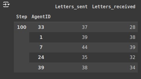
Figure 5. Number of letters sent and received by a selction of agents, at step 100 of the simulation
You’ll see that the DataFrame’s index is pairings of model step and agent ID. You can analyze it the way you would any other DataFrame, e.g. by following the tutorial on Visualizing Date with Bokeh and Pandas. Let’s get a histogram of agent’s letters sent at the model’s end:
end_letters = agent_letters.xs(99, level="Step")["Letters_sent"]
end_letters.hist(bins=range(agent_letters.Letters_sent.max() + 1))
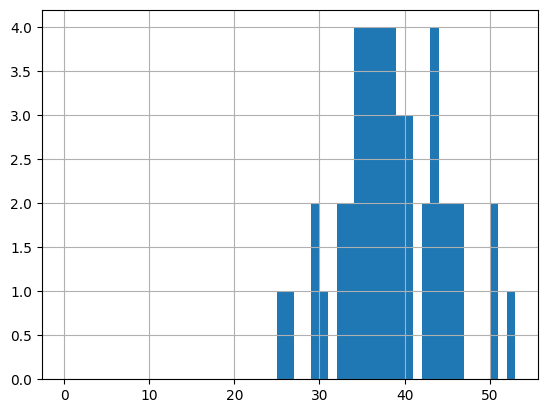
Figure 6. A histogram of agent’s letters sent after 100 steps of simulating the model
You can also use pandas to export the data to a CSV (comma separated value) file, which can be opened by any common spreadsheet application or opened by pandas.
If you do not specify a file path, the file will be saved in the local directory. After you run the code below you will see a file appear (agent_data.csv)
agent_letters.to_csv("agent_data.csv")
Having exported the data we can then apply several approaches to test the hypotheses that we encoded in the model. The goal to systematically test - or validate - a model is to check if the model actually represents what it is supposed to. This can range from simple testing of your expectations versus the outputs, to analyzing the internal consistency of the model, over a detailed exploration of the possible parameters of your simulation (a so called parameter space), to a detailed calibration to available empirical data.[^663 Mehdizadeh et al 2022, p. 8-9, despite coming from the realm of mobility studies, offer a sensible differentiation of various validation methods as well as a good example into how Agent-based models are evaluated in other fields]
In our case, we should check if changing the model parameters leads to data that corresponds to our expectations, e.g., if we would use a different random distribution for the letter sending, we would expect to see a different distribution of received letters.
Another option lies in the idea of Network Morphospaces[^667], which is a type of parameter space analysis. For this approach we would run the model several times for every possible parameter set and record the resulting output. Parameters could, e.g., change the likelihood of sending a letter in each round, vary the range of finding neighbors, or change the importance of the similarity of letter content to what the receiver’s mental state is in each round. Together with measures of the resulting output, e.g., fitting it to a distribution, or in the case of network output, its centralities, the parameter sets yield a fingerprint of each simulation run, which can be used to create an abstract embedding space. By including empirical data, in our case of historical networks, into such a space, one can observe which parameter sets bring the simulated outcome closer to the observed outcome. By adapting both the way how hypotheses are encoded in the model and what simulation parameters are chosen, one can bring the model outcome closer to empirical findings.
Bonus question 4: Try to plot the time series of received letters for a single agent. Hint: You can use the same way of accessing the dataframe, but on the level of the AgentID. Instead of using dataframe.hist(), use dataframe.plot().
Bonus question 5: So far, we have collected only counts of sent and received letters. How could we capture the sending of a letter as a link between sender and receiver? Can you create a model reporter that writes this information into a letter ledger? Hint: The information should be stored in a model variable, which is appended with every agent’s letter sending step. You can have a look in the published Historical Letters model 1.1.0.
2.5.7 Visualization and Interactive Features of Mesa
More recently, the mesa contributors have introduced a possibility to control and visualize a simulation directly in a Jupyter notebook.
For this, we need to define three components: the portrayal of the agents in the visualization, what parameters of the model we want to control, and finally the visualization itself.
Additionally, for the portrayal we define the agents color and size. To have some visual cue on the model run, we change the agents’ color once they have received a certain number of letters.
def agent_portrayal(agent):
    color = "tab:blue"
    size = 5
    agents_letters = agent.letters_received
    if agents_letters > 5:
        size = agents_letters
    if agents_letters > 30:
        color = "tab:red"
    return {
        "color": color, "size": size,
    }
In the visualization, we want to be able to control the amount of agents that are generated. This is an integer number, which we allow to be changed from 10 to 100 agents in steps of one. The width and height of the grid will stay fixed in the simulation.
We additionaly introduce an option to switch between two modes of how the agents select neighbours for their letter sending. Both are randomly selecting from a list. If we select reinforce as True, the choice is weighted by the number of received letters of the neighbors.
if self.reinforce == False:
    other_agent = self.random.choice(cellmates)
else:
    weights = [x.letters_received for x in cellmates]
    if sum(weights) == 0:
        weights = None
    other_agent = self.random.choices(
        population=cellmates,
        weights=weights,
        k=1
    )[0]
If agents have already received some letters, the likeliness of receiveing more letters grows. In this way, we can allow agents to become, in a sense, more “famous”. This could be one simple possible mechanism to model why well known people like Christiaan Huygens seem to have gotten much more letters than others.
We also make it less likely for every agent to move in every step. For this, we introduce another weighted random choice, this time with fixed weight. Now agents will only move with a chance of 20%, whenever they draw a one.
if self.random.choices([0,1], weights=[0.8, 0.2], k=1)[0] == 1:
    new_position = self.random.choice(possible_steps)
    self.model.grid.move_agent(self, new_position)
To be able to initialize the agents with this new option we also have to add another parameter to the model itself. All together we get the following new definitions for agents and the model.
class LetterAgent(mesa.Agent):
    """An agent with letters sent and letters received."""

    def __init__(self, unique_id, model, reinforce=False):
        super().__init__(unique_id, model)
        self.letters_sent = 0
        self.letters_received = 0
        self.reinforce = reinforce

    def move(self):
        possible_steps = self.model.grid.get_neighborhood(
            self.pos, moore=True, include_center=False
        )
        if self.random.choices([0,1], weights=[0.8, 0.2], k=1)[0] == 1:
            new_position = self.random.choice(possible_steps)
            self.model.grid.move_agent(self, new_position)

    def send_letter(self):
        cellmates = self.model.grid.get_cell_list_contents([self.pos])
        if len(cellmates) > 1:
            if self.reinforce == False:
                other_agent = self.random.choice(cellmates)
            else:
                weights = [x.letters_received for x in cellmates]
                if sum(weights) == 0:
                    weights = None
                other_agent = self.random.choices(
                    population=cellmates,
                    weights=weights,
                    k=1
                )[0]
            other_agent.letters_received += 1
            self.letters_sent += 1

    def step(self):
        self.move()
        self.send_letter()


class LetterModel(mesa.Model):
    """A model with a certain number of agents."""

    def __init__(self, N, width, height, reinforce=False):
        super().__init__()
        self.num_agents = N
        self.grid = mesa.space.MultiGrid(width, height, True)
        self.schedule = mesa.time.RandomActivation(self)
        # Create agents
        for i in range(self.num_agents):
            a = LetterAgent(i, self, reinforce)
            self.schedule.add(a)
            # Add the agent to a random grid cell
            x = self.random.randrange(self.grid.width)
            y = self.random.randrange(self.grid.height)
            self.grid.place_agent(a, (x, y))

        self.datacollector = mesa.DataCollector(
            agent_reporters={"Letters_sent": "letters_sent", "Letters_received": "letters_received"},
            model_reporters={ "Letters_received": compute_received_letters}
        )

    def step(self):
        self.schedule.step()
        self.datacollector.collect(self)
We can now setup the interface parameters we want to be able to control in the visualization.
model_params = {
    "N": {
        "type": "SliderInt",
        "value": 50,
        "label": "Amount of agents:",
        "min": 10,
        "max": 100,
        "step": 1,
    },
    "reinforce": {
        "type":"Select",
        "value": False,
        "values": [True, False]
    },
    "width": 10,
    "height": 10,
}
The model can be run within a visualization using the currently experimental visualization based on the Solara package. With this package we can also define our own visualizations, e.g. using a histogram as introduced above.
import solara
from matplotlib.figure import Figure

def make_histogram(model):
    fig = Figure()
    ax = fig.subplots()
    letter_vals = [agent.letters_received for agent in model.schedule.agents]
    ax.hist(letter_vals, bins=10)
    solara.FigureMatplotlib(fig)
The simulation is called with the model to run, its parameters, the measures that should be visible and the chosen agent style.
Try to run the model for a while. Do the agent colors change?
from mesa.experimental import JupyterViz

simulation = JupyterViz(
    LetterModel,
    model_params,
    measures=[make_histogram],
    name="LetterModel",
    agent_portrayal=agent_portrayal,
)

simulation
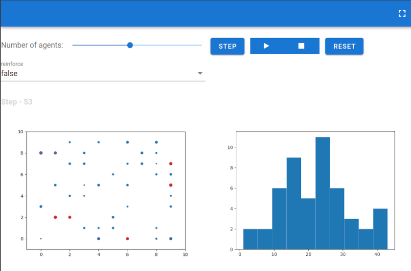
Figure 7. An image of an interactive interface for the simulation with multiple real-time visualizations
What difference do you observe in the visualization, when switching between reinforce True or False?
Bonus question 6: How could you use reinforement for the movement process? This would make more “famous” senders more likely to be the target of a movement process.
Part 3: A Summary, Open Questions and Next Steps
Now we have a relatively basic model for the process we wanted to depict, the exchange of letters during the time of the Republic of Letters. Our model has the following features:
- A grid-like space, the cells of which are occupied by Agents,
- Agents that can send each other letters,
- Agents that move about in space.
As well as those bonus features:
- Agents can send letters to others more than one cell away,
- A letter ledger, akin to an edge-list of a network,
- Agents moving purposefully in the direction of more ‘famous’ Agents, i.e., those who receive a lot of letters.
Of course, this model is still quite a distance away from being a plausible model of the Republic of Letters, but it has some of the most important base features you would expect from such a model.
Now the question remains how you could go on with this model, but also how to go on with Agent-based Modeling in general!
3.1 Suggestions for extending the model
You already may have come up with your own ideas for extending the model, but we want to give you at least some inspiration for further extensions. Importantly, we want to suggest to you some features that have strong connections to the historical subject matter and which raise some interesting modelling challenges:
- Implement a way for agents to “die” and new agents to be “born” during the simulation. In the real world, not only did some letter writers actually die at some point, but they also might have phases of letter writing activity.
- Think of a representation of the knowledge that is exchanged and how this should influence the other parts of the model. In the end, one of the most interesting aspects about the Republic of Letters is that it likely had a transformative impact on scientific activity in Europe. Try to envisage how this aspect could be introduced in and analyzed with this model!
- Implement an actual geographic space, rather than a grid. Space has some important repurcussions on movement and letter sending dynamics. Also, the Republic of Letters mainly featured people in the Low Countries and Northern Italy. Think about what geographical aspects of the Republic of Letters should be present in the model and how to implement them. To do this, maybe take a look at mesa-geo, a GIS (Geoinformation System) extension to the
mesapackage.
For more inspiration, you might also want look at our own extended version of this model!
3.2 Further Steps and Resources
At this point, we are finished with the tutorial but there is a lot more to learn not only about the technical side of things, but also the unique quirks as well as best practices of Agent-based modeling methodology.
For any technical questions, we suggest you head over to the documentation of mesa, which also features tutorials on advanced features, especially built-in javascript-based visualization methods. You can also head to youtube for a video tutorial in a similar vein like the official mesa tutorials.
We also want to at least mention some of the key methodological aspects we cannot cover here.
First of all, there is the aspect of documentation and publishing of Agent-based Models. There is a still developing, but already quite established method of formally documenting the complex beasts those models are, which is called ODD (‘Overview, Design Concepts, Details’)22. This is a document that lists all the features and design intentions of your model, with the explicit aim that others should be able to replicate a version of your model just from the ODD. Writing up an ODD can also help yourself understanding your goals as well as possible gaps in your model, too!
Many models are published on the website CoMSES, hosted by the Network for Computational Modeling in Social and Ecological Sciences. We recommend you to give their model library a browse, but also to publish your own models’ code and ODD there. While it is not a platform geared towards historians (such a platform sadly does not exist, yet) it is a great place that encourages reproducability, reusability and even gives the opportunity for peer review.
Many models are published in early, unfinished states to gather feedback. Models are often developed collaboratively in this way, and you should not hesitate to publish preliminary work in a non-peer review venue such as this. This strong tradition of collaboration and iterative, experimentative work can be a great asset to your own modeling.
3.3 Final Remarks
Agent-based Modeling for historians is still in an early phase. There is still a small - albeit growing! - number of people who apply simulation methods to historical research questions and there are many open questions left regarding the methods’ implications and prerquisites for historical inquiry.
The methodological criticism, which is so important for todays Digital History, is still just unfolding, but this also leaves much room for exiting discussion and discoveries.
Do not hesitate to get in touch with us if you want to be part of this discussion and if you want to help us build a community of practice around historical simulation methods!
Endnotes
New References: [^116]: Scheuermann, Leif (2022), Über die Rolle computerbasierter Modellrechnungen und Simulationen für eine digitale Geschichte, In Digital History. Konzepte, Methoden und Kritiken Digitaler Geschichtswissenschaft. edited by Karoline Dominika Döring, Stefan Haas, Mareike König, and Jörg Wettlaufer. Berlin; Boston 2022 (Studies in Digital History and Hermeneutics 6).
[^663] Mehdizadeh, Milad, Trond Nordfjaern, und Christian A. Klöckner. (2022). „A systematic review of the agent-based modelling/simulation paradigm in mobility transition“. Technological Forecasting and Social Change 184:122011, p.8-9. doi.
[^667] Avena-Koenigsberger, Andrea, Joaquín Goñi, Ricard Solé, and Olaf Sporns. “Network Morphospace.” Journal of The Royal Society Interface 12, no. 103 (2015): 20140881. https://doi.org/10.1098/rsif.2014.0881.
-
Hotson, Howard, and Thomas Wallnig, [Eds.] (2019), Reassembling the Republic of Letters in the Digital Age: Standards, Systems, Scholarship. Göttingen, Germany: Göttingen University Press. https://doi.org/10.17875/gup2019-1146. ↩
-
Ureña-Carrion, Javier, Petri Leskinen, Jouni Tuominen, Charles van den Heuvel, Eero Hyvönen, and Mikko Kivelä (2021), Communication Now and Then: Analyzing the Republic of Letters as a Communication Network. http://arxiv.org/abs/2112.04336. ↩
-
Miert, Dirk van (2014), “What was the Republic of Letters? A brief introduction to a long history.” Groniek, no. 204/5 (2014). https://ugp.rug.nl/groniek/article/view/27601. ↩
-
Schmitz, Jascha Merijn: Simulation. In: AG Digital Humanities Theorie des Verbandes Digital Humanities im deutschsprachigen Raum e. V. (Hg.): Begriffe der Digital Humanities. Ein diskursives Glossar (= Zeitschrift für digitale Geisteswissenschaften / Working Papers, 2). Wolfenbüttel 2023. 25.05.2023. Version 2.0 vom 16.05.2024. HTML / XML / PDF. https://doi.org/10.17175/wp_2023_011_v2. ↩
-
Gavin, Michael. Agent-Based Modeling and Historical Simulation. Digital Humanities Quarterly, 008(4):195, December 2014. http://www.digitalhumanities.org/dhq/vol/8/4/000195/000195.html. ↩
-
McCarty, Willard (2019). “Modeling the Actual, Simulating the Possible.” In The Shape of Data in the Digital Humanities: Modeling Texts and Text-Based Resources / Edited by Julia Flanders and Fotis Jannidis., edited by Julia Flanders, Fotis Jannidis, and Willard McCarty. London: Routledge. https://www.taylorfrancis.com/books/9781315552941. ↩ ↩2
-
Wendell, Augustus, Burcak Ozludil Altin, and Ulysee Thompson (2016), “Prototyping a Temporospatial Simulation Framework:Case of an Ottoman Insane Asylum,” 485–91. Oulu, Finland. https://doi.org/10.52842/conf.ecaade.2016.2.485. ↩
-
Winsberg, Eric (2019), “Computer Simulations in Science.” In The Stanford Encyclopedia of Philosophy, eds.: Edward N. Zalta. Metaphysics Research Lab, Stanford University. https://plato.stanford.edu/archives/win2019/entries/simulations-science/. ↩
-
Schmitz, Jascha Merijn and Buarque, Bernardo Sousa. 2023. “Introduction to Agent-based modeling for Historians”, ModelSEN Compendium. https://modelsen.gea.mpg.de/jupyterbooks/book/abmintro/. Accessed: June 3rd, 2024. ↩
-
Levison, M, R Gerard Ward, and John W Webb,(1972), “The Settlement of Polynesia: A Report on a Computer Simulation.” Archaeology & Physical Anthropology in Oceania 7, no. 3 (1972): 234–45. ↩
-
Wachter, Kenneth W., Peter Laslett, and Eugene A. Hammel (1978), Statistical Studies of Historical Social Structure. Population and Social Structure: Advances in Historical Demography. London: Academic Press. ↩ ↩2
-
Wachter, Kenneth W., and Eugene A. Hammel (1986), “The Genesis of Experimental History.” In The World We Have Gained: Histories of Population and Social Structure. Essays Presented to Peter Laslett on His Seventieth Birthday., edited by Lloyd Bonfield, Richard M. Smith, and Keith Wrightson. Oxford: Basil Blackwell Ltd. ↩
-
Epstein, Joshua M., and Robert Axtell (1996), Growing Artificial Societies. Social Science from the Bottom Up. Washington: Brookings Institution Press. ↩
-
Gooding, Tim (2019), “Agent-Based Model History and Development.” In Economics for a Fairer Society, by Tim Gooding, 25–36. Cham: Springer International Publishing. https://doi.org/10.1007/978-3-030-17020-2_4. ↩
-
Mitchell, Melanie (2011), Complexity: A Guided Tour. Oxford: Oxford University Press. ↩
-
Graham, Shawn. An Enchantment of Digital Archaeology: Raising the Dead with Agent-Based Models, Archaeogaming and Artificial Intelligence. Digital Archaeology: Documenting the Anthropocene 1. online: Berghahn Books, 2020. https://doi.org/10.1515/9781789207873. ↩
-
Brughmans, Tom, and Andrew Wilson, eds. Simulating Roman Economies: Theories, Methods, and Computational Models. Oxford: Oxford University Press, 2022. https://doi.org/10.1093/oso/9780192857828.001.0001. ↩
-
Wachter, Laslett and Hammel 1978, p. xix ↩
-
Comer, Kenneth W. “Who Goes First? An Examination of the Impact of Activation on Outcome Behavior in AgentBased Models.” George Mason University, 2014. http://mars.gmu.edu/bitstream/handle/1920/9070/Comer_gmu_0883E_10539.pdf. ↩
-
Unlike
mesa.modelormesa.agent,mesa.timehas multiple classes (e.g.RandomActivation,StagedActivationetc). To ensure context, time is used in the import as evidenced below withmesa.time.RandomActivation. You can see the different time classes at mesa.time. ↩ -
However there are more types of space to include
HexGrid,NetworkGrid, and the previously mentionedContinuousSpace. Similar tomesa.timecontext is retained withmesa.space.[enter class]. You can see the different classes atmesa.space. ↩ -
Grimm, Volker and Railsback, Steven F. and Vincenot, Christian E. and Berger, Uta and Gallagher, Cara and DeAngelis, Donald L. and Edmonds, Bruce and Ge, Jiaqi and Giske, Jarl and Groeneveld, Jürgen and Johnston, Alice S.A. and Milles, Alexander and Nabe-Nielsen, Jacob and Polhill, J. Gareth and Radchuk, Viktoriia and Rohwäder, Marie-Sophie and Stillman, Richard A. and Thiele, Jan C. and Ayllon, Daniel (2020). The ODD Protocol for Describing Agent-Based and Other Simulation Models: A Second Update to Improve Clarity, Replication, and StructuralRealism’ Journal of Artificial Societies and Social Simulation 23 (2) 7. https://doi:10.18564/jasss.4259. ↩